
This Application Guide outlines all the steps from sample preparation to data analysis for typical protein unfolding experiments on the C-Trap. This document strictly serves as a starting point for you to define your own experimental conditions and workflows. This guide can also be used for nucleic acid folding experiments (e.g. DNA hairpin, RNA hairpin, etc.). While LUMICKS’ has experience with these protocols, the outcome cannot be guaranteed and as always, the final decision and responsibility remain with the C-Trap users
Sample preparation
Construct design and assembly
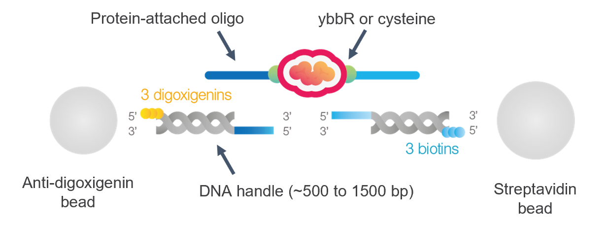
The protein of interest is generally functionalized with two ssDNA oligos and attached to dsDNA handles. Such a construct can be attached to two optically trapped beads to enable single-protein manipulation, force sensing and detection of fluorescently-labelled proteins (Fig. 1). The protein can be attached to DNA oligos using different strategies:
•Coupling of maleimide-modified oligos with two cysteine residues on the protein (either naturally present or introduced with point mutations). The position of the cysteines should be chosen so that they are surface-exposed and the functionalization does not interfere with folding [1] (see also LUMICKS kit).
•Coupling of CoA-modified oligos with ybbR tags added at the C- and N-termini of the protein [1] (see also LUMICKS kit).
•Other strategies involve cysteine crosslinkers [2], ssrAtag [3], HaloTag [4], SpyTag-Catcher [5].
Importantly, the attachment point of the handles to the protein has an impact on the direction in which the unfolding force can be applied and on which domains will be affected by such force. Once attached to the protein, the DNA oligos can be annealed to dsDNA handles with suitable overhangs. Depending on the length of the overhangs, a ligation step may be needed to stabilize the construct against stretching at high forces. More details on construct assembly can be found in the protocols associated with LUMICKS kits (where no ligation step is done, limiting the stretching forces to ~45 pN).
Suitable DNA handles for protein-folding experiments
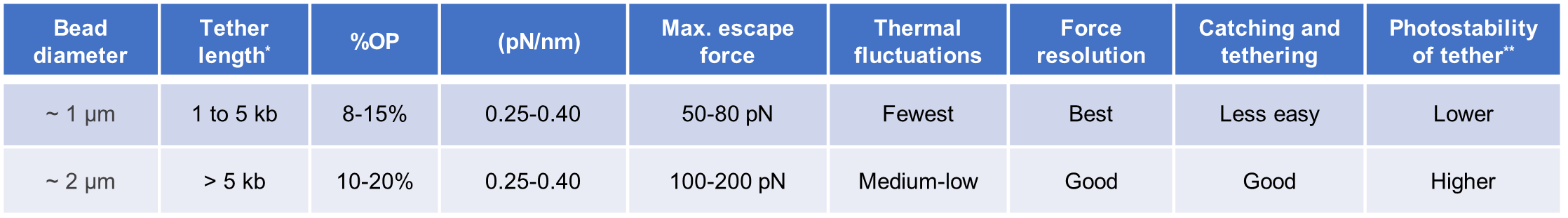
The length of the DNA handles should be chosen based on the experimental application. Shorter DNA handles (as short as 0.5 kb) display fewer thermal fluctuations, implying a better signal-to-noise ratio in the force and distance data. The standard LUMICKS kits for protein tethering offer two handle sizes: 1.5 kb for an easier tethering workflow, and 0.5 kb for the highest force &distance resolution. Conversely, assays involving fluorescence imaging require the handles to be long enough to resolve the fluorescence signal of the protein (or protein-bound molecules) from that of the beads (autofluorescence or non-specific binding of labelled molecules). The recommended handle size for fluorescence assays is 5 kb [6], preferably longer, while the shortest documented size is 2.5 kb [7]. For handle sizes below ~4 kb, the likelihood of a symmetrically labelled tether (e.g. biotin on both sides of the annealed tether) to bind on the same bead is very high. Therefore, these short tethers (<8 kb total) require different end labels, typically biotin and digoxigenin.
Buffer, beads and C-Trap settings
Buffers used in experiments with smaller beads (~ 1 μm) and shorter constructs (a few kb) can be supplemented with oxygen scavenger systems, such as glucose oxidase system to increase the photostability of the tether [1]. The bead material is usually polystyrene (easier to trap) or silica, and the coating is typically streptavidin (for biotinylated DNA handle) or anti-dig (for digoxigenated DNA handle). ~1 μm beads can be sonicated for 10-15 seconds in a water batch to disrupt large clusters before being used.
C-Trap operations
Preparation
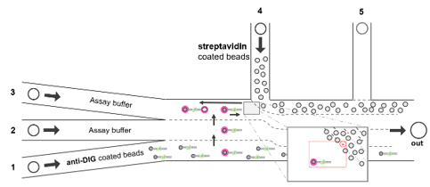
When working with small beads (~ 1 μm) and short constructs (up to 5 kb), the tethering process in the C-Trap is more difficult due to the much lower accessible surface of the beads. To increase the tethering efficiency, one side of the construct can be attached to a bead before the C-Trap experiment. This can be done using DNA handles with different labels (typically one with biotin and one with digoxigenin) and two bead coatings (streptavidin and anti-dig). The construct is pre-incubated at high concentrations with one bead type (restricting volumes to a few μLs). After some time that can vary from a few minutes to one hour depending on bead size/density, DNA concentration, and total volume, the mixture is diluted and loaded in one microfluidic in e.g. channel 1 of the C-Trap (Fig 2).
Tethering workflow
When two different bead types (e.g. anti-digoxygenin, AD, and streptavidin, SA) are used due to the short tether, one type of beads is pre-attached to the DNA. The recommended workflow is listed below and illustrated in Fig. 2.
- AD beads are loaded in channel 1and SA beads in channel 4. Channels 2 and 3 are loaded with buffers. Make sure to draw the bead templates correctly (see how to draw templates and make sure you trap a single bead in the Tips & Tricks section).
- The traps are positioned diagonally and far away from each other in the trap 1 range of motion. They are then moved to channel 1, where one AD bead is caught in trap 2 under flow (0.1 bar works best for small beads).
- The traps are moved near to the channel 4 junction to expose trap 1 (but not trap 2) to the flow of SA beads.
- After catching one SA bead in trap 1, the traps are moved to the buffer channel. The flow is stopped.
- The traps are horizontally aligned (with trap 1 on the right) and the distance between the beads is set to ≥ 5 μm (or at least 5 times the bead diameter).
- After calibrating and zeroing the forces, piezotracking (PT, see note below) is activated. On the left screen, switch to PT visualization in the FD curves by choosing the high frequency HF channels. Repeat step 6 for every bead pair.
- The right bead is moved using trap 1 towards the left bead. Trap 1 is moved back and forth to tether the DNA while checking the FD curve. It is useful to plot the theoretical FD curve on Bluelake as a reference, however, keep in mind that PT will intrinsically have some distance offsets (which can be accounted for later in data processing), therefore the displayed PT distance may be significantly off from the theoretical model. For short DNA constructs between 1 and 5 kb, flow is not needed for tethering.
- When a single tether is formed, the relevant data can be recorded (see tips & tricks, and data recording sections further).
- When data acquisition is completed on the current bead pair, the tether can be broken, and a baseline can be measured by recording an FD curve that covers at least the same distance range as in the relevant FD curves. Alternatively, the baseline curve can be recorded during the very first bead approach right after step 6.
- Once per session, or anytime the bright-field templates are changed, a longer baseline curve should be recorded covering a longer distance range (e.g. 2 to 5 μm) where both PT and video tracking are functioning correctly. This dataset can be used in post processing for distance calibration purposes. This can also be accomplished in step 7, using the baseline curve from the initial approach.
When using one type of beads only and a DNA construct with the same labels (e.g. biotin) on both handles, the pre-incubation step is skipped, and the tethering is performed in situ entirely in the C-Trap using the standard DNA workflow (beads are loaded in channel 1, the DNA construct in channel 2, and the buffer in channel 3, see LUMICKS kit protocol). This is only possible when the handles are 4 kb or longer (total tether length of 8 kb or longer).
Note on piezotracking (PT)
The C-Trap can measure distances by using the bright-field images of the beads (video tracking), or by means of tracking (PT) that is, by tracking changes in trap position and forces. The latter strategy is particularly suited for protein-folding assays with short tethers because it can push the time resolution of distance data up to the kHz range and because video-tracking is not effective when the beads are too close (when the distance is < ~1.5 μm). For more details on the practicalities and the theory of PT, see the material attached to the example python analysis notebook.
Data recording: force-distance curves
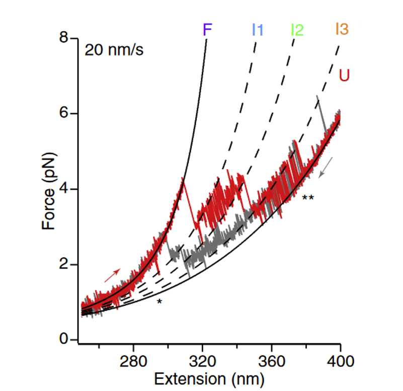
The tether can be stretched by moving trap 1 at constant velocity. An FD curve can be recorded during trap 1 movement using the appropriate Bluelake widget. The FD recording should start when the tether is relaxed and the protein is folded (typically, force ≤ 1 pN after baseline subtraction). Upon pulling, the FD curve initially follows the model for the DNA handles. When the force has increased sufficiently, the mechanical stress causes one protein domain to suddenly unfold. This releases a certain number of amino acids, increasing the tether length and resulting in a momentary drop in force. The pulling continues until all domains are unfolded, yielding a characteristic saw-tooth pattern in the FD curve (Fig. 3). The unfolding forces are a measure of the mechanical stability of protein domains, while the changes in extension relate to the size of conformational changes in the pulling direction (in many cases, this corresponds to number of amino acids released in the unfolding).
When full unfolding is achieved, trap 1 is stopped and its movement can be reverted by moving it at the same constant velocity in the opposite direction, relaxing the tether and allowing the collapse of the protein chain, and in some cases, its refolding. The trap can be stopped at the same point were the stretching started. Please note that protein refolding might occur at different (typically lower) forces than the unfolding or might not happen at all within the experimental time window.
After reaching the initial point, a new stretch-relax cycle can be performed. The newly acquired FD curve will likely show a different saw-tooth pattern due to the stochasticity of the unfolding process. Furthermore, by testing if the low-force part of the new FD curve (before any unfolding) overlaps with the FD from the first pulling, one can deduce if the protein fully refolded or not in the previous relax phase. If the refolding is a slow process, a pause can be added at the end of the relax phase to allow more time for the collapsed chain to refold. By measuring the refolding yield as a function of the waiting time, the refolding rate can be determined. The above-described workflow with cyclical stretch-relax phases can be automated in Bluelake by using the ping pong feature or automation scripting.
Data recording: time traces at constant trap distance
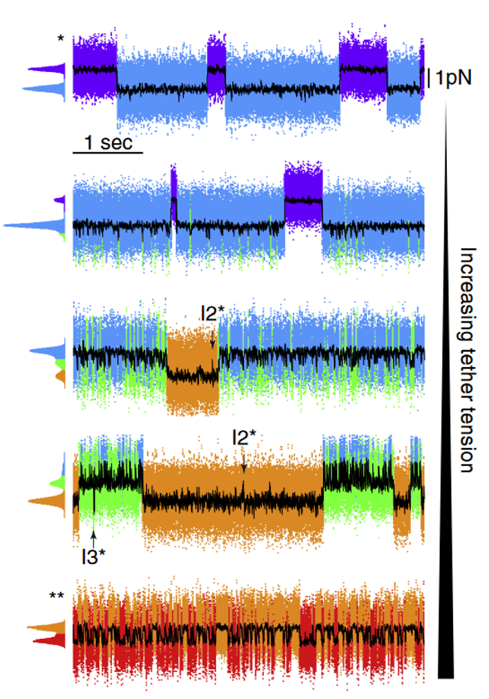
The folding and unfolding rates between two conformations critically depend on the force applied to the protein. In the case where unfolding and refolding happen on similar time scales and within the experimental time window, more kinetic (and thermodynamic) information can be obtained by monitoring the force readout while keeping the traps at constant distance (in contrast to constant-force, see note below). Under this regime, the force and extension will jump between different levels corresponding to different folded states of the protein (Fig.4). By measuring the dwell times in the different states, the unfolding and refolding rates between them can be extracted. For this to work, it is imperative that the trap-to-trap distance remains stable within the observation time. Failure to achieve this results in a drift in the force levels over time. The recording can be repeated at different trap-to-trap distances (implicating different average forces) to alter the equilibrium between folded states and extrapolate the energy landscape of the protein in absence of force (Fig. 4, see also data analysis section). The force and distance traces can be marked in the Bluelake timeline for exporting and data analysis.
Note on constant-force measurement
A constant force measurement requires active force feedback to change the trap position for every unfolding/refolding event. The force feedback should be faster than the unfolding/refolding dynamics. Since these dynamics are typically very fast, using force feedback is usually not an option. In addition, even a well-tuned force feedback mechanism will likely introduce artifacts and extra noise due to its active nature.
Data exporting
Although Bluelake displays a Distance channel, for more accurate data, it is highly recommended to recalculate the Distance in post-processing using the raw force and trap 1 position data. The following channels should be exported: all HF Forces (1X, 1Y, 2X, 2Y), Distance 1 (i.e. the distance measured with video tracking) and Trap position (1X, 1Y). Although not strictly needed for the analysis, it can be useful to also export the LF Forces, Distance, Bead positions and Tracking Match Score, and Power controls. For fluorescence assays, the Photon Counts and Confocal Diagnostic (shutters and excitation lasers) should also be selected.
Tips & tricks
Make sure to properly perform force calibration. Assign the correct bead template and diameter to each trap. Use 200 points per block and enable hydrodynamic correction. The fitting range can be adjusted to cut out noise peaks, provided the corner frequency is well within the fitting range. The fitting range should at least include data from ~5x lower than the corner frequency to 5x larger than the corner frequency. Trap stiffness should be around 0.3-0.4 pN/nm and the difference between its X and Y components for the same trap should be < 15%. Furthermore, the relative error on the fitted corner frequency (err_fc, after selecting to show the detailed fit results), should be less than 10% of the corner frequency.
Draw the bright-field template as centered with the beads as possible to reduce the systematic errors in distance measurements (which can always be accounted for in post-processing) and facilitate the workflow
Keep a consistent workflow: e.g. use trap 1 saved positions for bead catching, calibration, and tethering, but also for the start and end positions of the FD curves, keep trap 2 static, etc.
Make sure to trap single beads. Trapping the correct bead is typically more difficult with smaller beads. After repeatedly catching beads, the most commonly caught beads should be the correct one and should then be used for the bright-field template. When unsure about whether a single bead or more were caught, one can shutter the trap in absence of flow and check how many beads are released. Once a bright-field template is properly set (on the correct bead) a high matching score (>95% typically) can then be used as a diagnostics for the correct single bead.
Choose an appropriate pulling speed when recording FD curves. The trap velocity should be scaled to the effective length of the tether to allow resolution of the unfolding event(s). A good starting value is 50 nm/s. Please note that the average unfolding force depends on the pulling velocity, with typically higher unfolding forces when using faster pulling speeds.
If the tethering efficiency is too low, you can increase the DNA/bead ratio and/or the waiting time in the pre-incubation step. If this is not effective, or the tethers break at very low forces, there might be a problem with the assembly of the construct, possibly due to an ineffective protein labelling or ligation step.
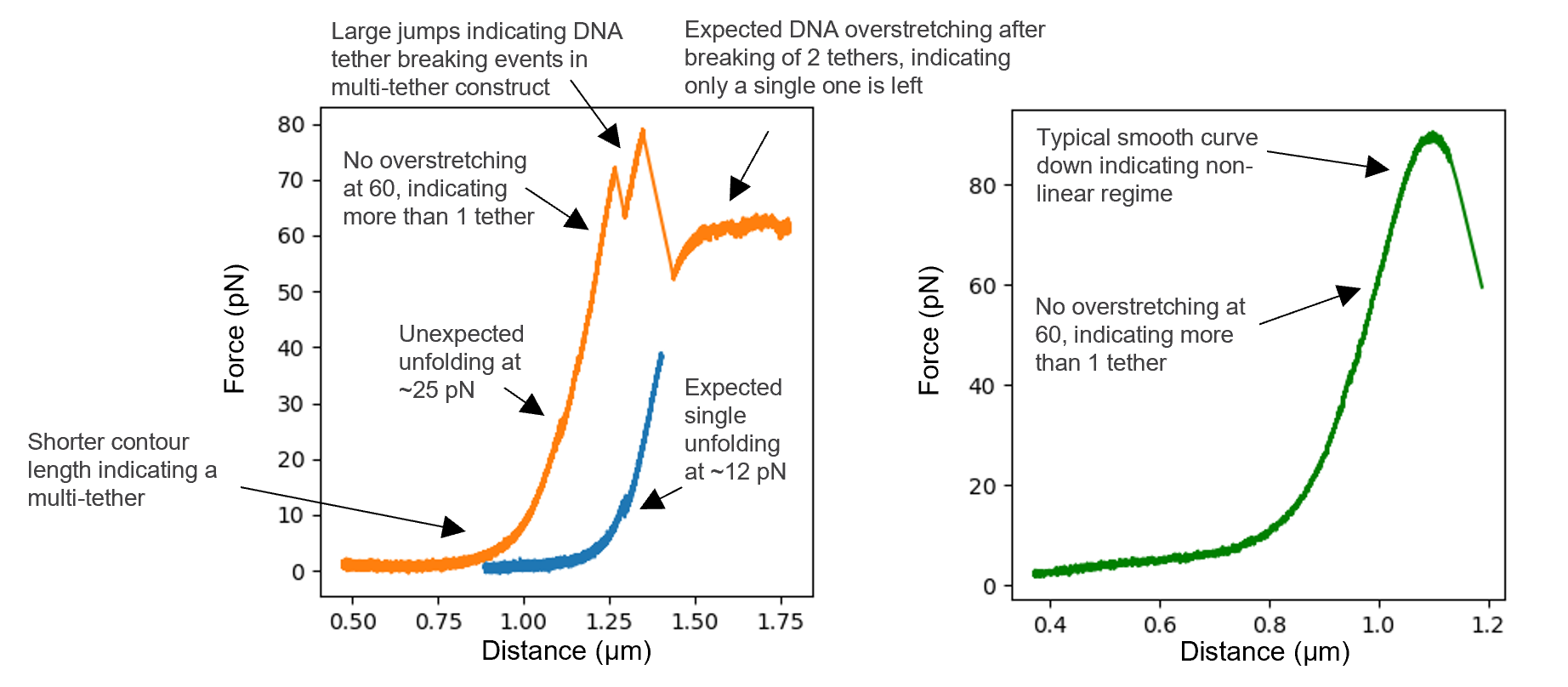
Make sure to work with single tethers. To increase the chance of getting single tethers, you can optimize the DNA/bead ratio in the pre-incubation step, as well as the distance of the bead approach in the tethering process (step 7 in the workflow). The theoretical FD curve on Bluelake can also serve as a reference. However, there is typically a distance offset between the PT and the real distance depending on how centered the bright-field templates were drawn. While this offset is typically fairly constant within a single experimental session (provided the templates are not changed), it can still vary between repeats. Nevertheless, after forming a few tethers, one should be able to effectively identify single tether from multiple tethers within a single experimental session despite the offset. For multiple tethers, the contour length will be shorter, and the steepness of the slope after the contour length may have a slightly steeper slope (the steepness is not always noticeable). The most accurate way to determine if it is more than one tether is to stretch the tether to the DNA overstretching plateau(~55-65 pN, Fig. 5, left). This is however not always practically possible depending on the stability of the construct (specifically, the ligation process) and the trapping settings (in particular, the trap stiffness, see next point for more details). Another tip is to look at discontinuities in the FD curves and determine if they are consistent with the expected unfolding events. FD curves with much larger jumps in extension than expected are likely resulting from multiple and/or improperly assembled tethers breaking (Fig. 5, left).
Make sure to stay in the linear regime of the trap, where F = kx holds. Depending on the bead size and power used (and the resulting stiffness), these settings determine the highest force achievable while remaining in the linear range. A typical sign of forces beyond the linear regime is shown in Fig. 5, right, where there is a clear bell-shaped smooth curve at higher forces in contrast to the typically jagged DNA overstretching plateau.
Trap1+2z position and the objective collar setting may both significantly impact your measurements. Be mindful of this when optimizing or changing the experimental conditions
If you encounter issues with even flow, clogging or bubbles, please find more information in this troubleshooting article
In certain cases, for example, when using two beads of different material, or when you want to tune the stiffness of one trap compared to the other, you can always change trap 1 split to achieve the desired outcome.
Data analysis
FD curve analysis
Two preliminary steps are needed before any further analysis of the FD curves (see tutorial notebook where the FD curve analysis workflow is demonstrated with DNA hairpin data, which are conceptually similar to protein unfolding data):
- Piezodistance (if used) is re-calculated by using a baseline curve recorded for this purpose on one representative bead pair: trap 1 mirror voltage is calibrated against the video-tracking distance to increase tracking accuracy. In certain cases, with longer handles and slower folding dynamics, the distance from bright-field image tracking at over 100 Hz may be suitable without the use of any piezotracking (i.e. piezodistance).
- The baseline force is subtracted from its corresponding FD curve.
In the corrected FD curves, the unfolding forces can be immediately obtained as the force value right before the discontinuity. The FD curves can also befitted with suitable models to determine the length of the unfolded domains. The curves are split into different segments where the folding state of the protein is constant. The very first segment, before any unfolding occurs, can be modelled as a single extensible Worm-Like Chain (eWLC) to account for the mechanical properties of both dsDNA handles (the contribution of the folded protein is typically neglected). Every subsequent segment is then modelled as the sum of the same eWLC for the handles and a second WLC (non-extensible) with another set of parameters to account for the different mechanical properties of the unfolded polypeptide chain. If multiple unfolding steps occur, each FD curve segment is assigned with the same parameters except for the contour length of the polypeptide chain, which is allowed to increase at any subsequent unfolding step (see the extended FD curve fitting documentation). The change in polypeptide contour length upon a certain unfolding event can be converted in the number of amino acids involved in the unfolded domain or can be used to quantify changes in protein conformation in the pulling direction (when there is no full unfolding). Once the fitting is completed, the resulting parameters should be thoroughly scrutinized:
- The DNA contour length should match that of the two handles – if not, a manual offset can be added.
- The total polypeptide contour length should be compatible with the size of the protein.
- The mechanical properties of DNA should be consistent with literature. If needed, the mechanical properties of the polypeptide can be fixed.
- For meaningful comparisons, the fitting parameters should be consistent between different FD curves of the same condition.
The average unfolding force increases with the loading rate, which is related to the pulling speed but also includes the contributions from the trap stiffness and tether stiffness. By recording FD curves at different pulling velocities (thus different loading rates), one can get a distribution of unfolding forces vs loading rates. Following the model developed by Evans and Ritchie, the unfolding force vs the logarithm of the loading rate can be fit to extract the unfolding rate at zero force and the distance to the transition state [8]. As for the folding rate, one can perform quenching experiments where after unfolding, the tether is relaxed for a specific amount of time until the protein refolds. The relationship between the waiting time and the refolding fraction can then be used to get the folding rate at zero force [9].The free energy of folding can also be obtained from FD curves using Crook’s fluctuation theorem. The folding and unfolding work energy (area under the curve) can be obtained and their distributions compared to extract the free energy of folding [1].
Constant trap distance analysis
Force (or distance) time traces recorded at constant trap positions and showing transition between different folding states (as in Fig. 4) can be analyzed to determine the unfolding and refolding rates. This analysis requires first the assignment of the different force (or distance) levels to a fixed number of folded states. This can be done using Hidden Markov Models. Please note that careful downsampling of the raw data is required to avoid introducing processing artifacts. The trace is then segmented into portions where the protein is in the same state before switching to a different one. For each segment, the dwell time, is calculated. In case of a two-state system, the dwell-time distributions of each state are fitted with exponential functions to determine their lifetimes and, consequently, the unfolding and refolding rate constants [1][10]. When more than two states are involved, a new dwell-time analysis is carried out for each possible transition between pairs of states at equilibrium to retrieve the corresponding rate constants. Please note that dwell-time distributions might require more than one exponential function for a satisfactory fitting. The obtained unfolding and refolding rates can be used to estimate the difference in free energy (i.e. the relative stability) and the energy barriers between folding states, thus reconstructing the energy landscape of the protein. The experiments can be repeated at different trap distances (and, consequently, different average forces), to assess the effect of external forces on the landscape. By using the Bell’s model, these different-force data can be used to extrapolate the rate constants and the energy landscape at zero force [1][10].
References
Examples with RNA hairpin:
Additional review:
Mora et al., The nanomechanics of individual proteins, Chemical Society Reviews, 2020
